Quadruped Locomotion

I implemented locomotion for a quadruped in MATLAB. I specifically implemented a walking gait and used that for forward, backward and lateral movement. Below, I elaborate on the math and coding required for the walking gait, which sets the foundation for more complicated locomotion like running and jumping.

Background

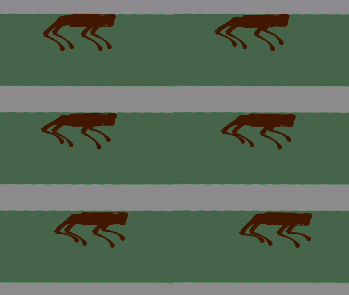
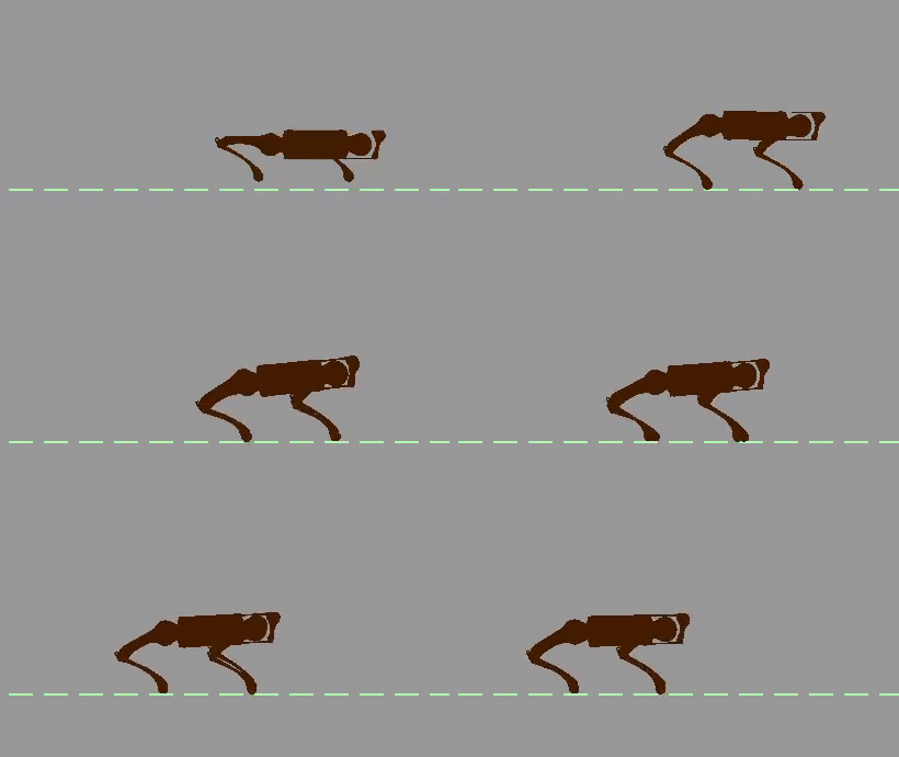
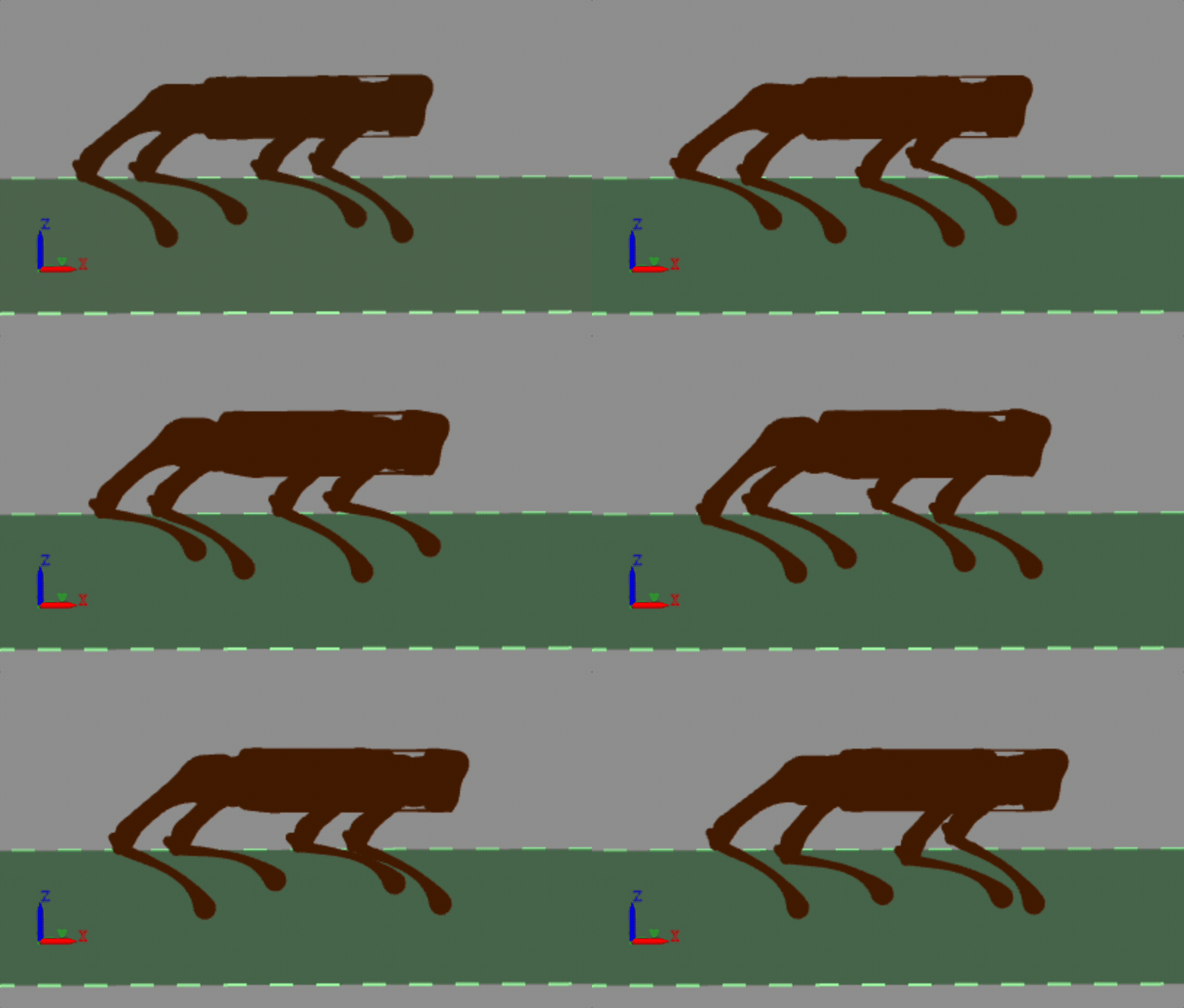
The walking gait is a coordinated movement between the legs of the robot that allow it to move forward along the x-axis. The gait consists of two operating modes. The first is the leg swing where the robot moves two diagonally opposite front and rear legs forward in an arc. This is shown in the animation below. The second is standing, which is when other two diagonally opposite front and rear legs balance and push the body forward. Both operating modes exist at every timestep and each calculate the torques required for the legs differently. Below I outline some of the math involved to generate the motor torques in each mode.

• Leg Swing
• Standing

Leg Swing

For the leg swing, the only goal is to move the feet of the quadruped in an arc forward. The diagram below illustrates this.

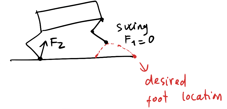
The steps for doing the above are the following:

1. Calculate the final foot position for each leg
2. Get the trajectory for the foot for the final position
3. Calculate and apply the torques to move the foot along the calculated trajectory

Step 1

For the first step, the final foot position is calculated using equation (2) below. The terms in the equation are the following:

$T_{stance}$ - The desired time it takes for a single step.

$V_{COM}$ - The velocity of the center of mass of the quadruped in the x-direction

$V_{desired}$ - The desired velocity of the center of mass of the quadruped in the x-direction

$Z_{COM}$ - The desired height for the center of mass of the robot

$g$ - The acceleration due to gravity

$P_{hip}$ - The location of the hip of a leg along the x-axis

$P_{foot}^{d}$ - The location of the foot along the x-axis

The two terms to note in the equation above are $\frac{T_{stance} \cdot V_{COM}}{2}$, which is the feedforward term and $K_{step} \cdot (V_{COM} - V_{desired})$, which is the feedback term. The feedback term is important to either add or subtract to the feedforward term to increase or decrease the speed of the robot. This term is positive when $V_{COM}$ is greater than the desired velocity and consequently the next foot position goes further in front to act as a brake. When $V_{COM}$ is lower than the desired velocity of the body, the next foot position is shorter, resulting in a speed up.

Step 2

The next step is to get a trajectory for the foot from the current position to the desired position. I chose a parabolic trajectory for the foot to move along like in the image below. Since the robot is moving along the x-axis, the trajectory is in the x-z plane. I use the equation (3) below with the total time the foot arc should take ($T_{swing}$) as a root to get a parabolic equation between 0 and $T_{swing}$ and multiply by a scaling factor to change the max height for the z coordinate. The x coordinate is simply $\Delta P_{foot} \cdot \frac{t}{T_{swing}}$

Step 3

The last step is more involved and requires getting the forces applied to each foot of the leg to get to a point along the parabola, and using that to calculate the joint torques.

To get the forces for the foot of each leg, I use a PD controller that is applied at every timestep. The PD controller equation (4) is below.

$P_{foot}$ - This is the cartesian coordinates of the foot at the current timestep.

$P_{foot}^{d}$ - This is the cartesian coordinates of the desired foot position along the calculated parabola for the current timestep. The x and z coordinates are updated while the y coordinate is the same as for $P_{foot}$

$\dot P_{foot}$ - This is the velocity of the foot at the current timestep.

$\dot P_{foot}^{d}$ - This is the desired velocity of the foot. The x velocity is constant at $\Delta P_{foot} / T_{swing}$. The y velocity is 0 and the z velocity is the time derivative of equation 3.

Once the forces for the foot are calculated, they need to be converted to torques because that control input for the quadruped. The torques can be calculated using the equation (5) below.

$J_{i}(q)^{T}$ - This is the transpose of the jacobian of the forward kinematics for a leg. The forward kinematics is simply an equation mapping the 3 joint angles of a leg to cartesian coordinate in the robot’s frame.

$R^{T}$ - This is the transpose of the rotation matrix for the robot

$F_{i}$ - The calculated force for the foot.

The Matlab code for computing the Jacobian can be found below. The function takes in angular velocities for the joints of a leg as well as an index representing the leg and returns the Jacobian for that leg.

function J=computeLegJacobian(q,leg)
    l1=0.045; % hip length
    l2=0.2; % thigh length
    l3=0.2; % calf length
    if leg==1 || leg==3 % left leg has sideSign 1
        sideSign=1;
    else
        sideSign=-1; % right leg has sideSign -1
    end
    J = zeros(3,3);

    s1=sin(q(1)); % for hip joint
    s2=sin(q(2)); % for thigh joint
    s3=sin(q(3)); % for calf joint
    
    c1=cos(q(1)); % for hip joint
    c2=cos(q(2)); % for thigh joint
    c3=cos(q(3)); % for calf joint
    
    c23=c2*c3-s2*s3;
    s23=s2*c3+c2*s3;
    
    J(1,1)=0;
    J(2,1)=-sideSign*l1*s1+l2*c2*c1+l3*c23*c1;
    J(3,1)=sideSign*l1*c1+l2*c2*s1+l3*c23*s1;
    
    J(1,2)=-l3*c23-l2*c2;
    J(2,2)=-l2*s2*s1-l3*s23*s1;
    J(3,2)=l2*s2*c1+l3*s23*c1;
    
    J(1,3)=-l3*c23;
    J(2,3)=-l3*s23*s1;
    J(3,3)=l3*s23*c1;
 end

Standing

The goal of the standing operating mode is to use the opposite diagonal legs on the ground to get the body to move forward while balancing. This requires finding the Ground Reaction Forces (GRFs) for the two feet on the ground to accomplish the goal. These are the forces that affect the quadruped when the feet apply forces to the ground. The diagram below shows this for a 2D quadruped.

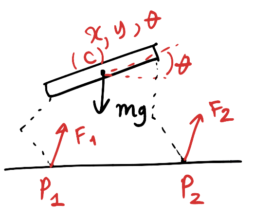
From these forces, we calculate the joint torques for the legs. There are three steps to effectively calculating these forces and is quite involved. I will give a broad summary of the math involved in these steps. The three steps are:

1. Linearize the quadruped dynamics
2. Formulate model predictive control (MPC) matrix equation
3. Use quadratic programming to optimize forces that satisfy MPC equation

Step 1

The first step requires finding a linearized model for the robot dynamics. This allows for predicting the next state after applying control input to the robot, which ultimately allows for finding the control input the gets the robot to the desired state.

A linearized model is shown in equation (6) below where $X$ is the robot state, $u$ is the control input and $\dot X$ is the state derivative while $A$ and $B$ are matrices that allow for a linear transformation.

The control inputs $u$ as shown are the ground reaction forces in the $x$, $y$, and $z$ directions for the 4 feet. They make up the vector below.

The state $X$ is the following:

$P_{3 \times 1}$ - The cartesian coordinates of the robot

$\theta_{3 \times 1}$ - The euler angles of the robot

$\dot P_{3 \times 1}$ - The velocities of the robot body

$\omega_{3 \times 1}$ - The angular velocity vector for the robot. The vector is the axis of rotation and the magnitude is the angular velocity at which it is rotating around that axis

$g_{1 \times 1}$ - The acceleration due to gravity

The state $\dot X$ is the following and represents the dynamics of the quadruped body.

$\dot P_{3 \times 1}$ - The velocity of the robot body.

$\dot \theta_{3 \times 1}$ - The time derivative of the euler angles. This requires a tranformation matrix that linearizes around the yaw ($\phi$). This is a simplification because the robot does not rotate much along the other two rotational axes.

$T(\phi)_{3 \times 3}$ - The transformation matrix

$\ddot P_{3 \times 1}$ - The acceleration of the body. The related variables to calculate this are $m$ for the mass of the robot body, $\vec{F}_{i}$ for the forces vectors for all the legs in the world frame and $\vec{g}$ for the gravity vector in the world frame

$\dot \omega_{3 \times 1}$ - The rotational acceleration. The related variables to calculate this are $R$ for the rotation matrix of the robot, $I_{b}$ for the moment of inertia of the robot in its frame and $\vec{r}_{i}$ for the vector from the center of mass of the robot to a foot

$\dot g_{1 \times 1}$ - The derivative of the acceleration due to gravity (jerk)

With the equations above representing $\dot X$, the matrix equation can be written with $A$ and $B$ below.

$S(\vec{a})$ - This is a skew-symmetric operator that turns a 3D vector ($\vec{a}$) into a matrix like below. This is so that cross product $ \vec{r}_{i} \times \vec{F}_{i}$ can be achieved by matrix multiplication.

Step 2

Model predictive control is simply finding a series of $m$ control inputs over $n$ timesteps that gets the desired state at each timestep. For my implementation, I did prediction for 12 control inputs ($F_{x}$, $F_{y}$, $F_{z}$ for 4 legs) MPC over time horizon of 10 timesteps with each timestep being 0.03 seconds. For illustrating the math below, I will show that calculation for 3 timesteps in the future.

The linearized model for 0.03 seconds is illustrated above. In MPC, the equality constraint equations simply show what the state at the end of each timestep should be using the linearized model. The constraint equations for three timesteps are below where $u[k+n]_{12 \times 1}$ is the control for each timestep and $x[k+n]_{13 \times 1}$ is the state for each timestep and A and B are from the linearized model from step 2.

Turning the above into a matrix equation results in the equation below where $X$ is a matrix of the states and the control inputs at each timestep.

Step 3

This last step is using quadratic programming to optimize a cost function representing the disparity between the desired state at each of the 3 timesteps and the predicted state and the magnitude of the control inputs. So the goal is to get to the desired states with the smallest control inputs. As a reminder, these control inputs are the forces that are applied to the feet of the robot. The quadratic cost function is the following:

$Q$ - This matrix are the gains in the cost function for the state and is the following diagonal matrix. For example, 40, 50, and 60 are the gains for prioritizing the position of the rigid body in the state to match the position in the desired state.

$R$ - This diagonal matrix are the gains for the forces for a single foot

The equation above needs to be simplified to put into a form that can be passed into $quadprog$ in MATLAB.

The $H$ and $f$ are matrices that are passed into $quadprog$ that are used in the following cost function $\frac{1}{2}XHX + f^TX$ and results in the equation (7) cost function. $H$ and $f$ are shown below for 3 timesteps.

$H$, $f$, $A_{eq}$, $B_{eq}$ are now enough to optimize for the control inputs. However, there are some constraints that should be placed on the control inputs. These are frictional constraints on the foot forces in the control inputs so that when the forces are applied to the foot, it doesn’t slip. These physics constraints for a single foot are below and are for the forces in the $x$, $y$ and $z$ directions.

Physics constraints above can be rewritten as inequalities below.

The physics constraints inequalities can be written in the matrix form below.

For $quadprog$ in MATLAB, if $A_{ineq}$ and $B_{ineq}$ are passed in, the expected relationship is $A_{ineq}X \leq B_{ineq}$. For 3 timesteps, $X$ is reiterated below, with each $u[k+i]$ being a vector of $F_{x}$, $F_{y}$, $F_{z}$ for each foot, which is why the dimension is $12 \times 1$.

To ensure $quadprog$ optimizes the control inputs ($u$) in $X$ with the physics constraints $A_{ineq}$ and $B_{ineq}$ need to be updated for each leg, then to each timestep.

The matrices for four legs are:

The final matrices for the four legs applied for each of the N = 3 timesteps results in the $A_{qp}$ and $B_{qp}$ shown below.

Finally, with $H$, $f$, $A_{eq}$, $B_{eq}$, $A_{qp}$, $B_{qp}$ now calculated, we can pass them into the $quadprog$ in MATLAB and get an optimized $X$. The 12 inputs at $u[k]$ after 39 (13N) rows in an optimized $X$, are the ideal control inputs to apply. The 12 inputs are made up of 3 control inputs/forces for each of the 4 legs. The forces for each leg are finally converted to motor torques using equation 5.