Robotics • RL (2023)
Neural Network Library
My goal was to implement an efficient neural network library from scratch and use it to create a Deep Q Network (DQN) RL agent to play Flappy Bird.

Neural Network Library
The are many approaches to developing a neural network library, I investigated two approaches, the computational graph approach and the layered approach. Both have their strengths and weaknesses. I implemented both and benchmarked them by training a DQN to successfully solve the Cart Pole problem.
Computational Graph
The computational graph approach, as the name suggests, is building a graph that represents all the computations taking place in a neural network, then implementing backpropagation over the graph to compute the gradients for all values involved in the computations.
My implementation is a reimplementation of Andrej Karpathy’s micrograd with some syntatic modifications. For a very thorough explanation you can refer to his video. Below, I summarize the implementation details.
Graph
For the computational graph an essential component is representing a computation. A computation is simply a mathematical operation between two values. In my case, these values are all floats. To represent these computations, I wrote a Value class in python to wrap values. The Value class contains a property for the float value, but also stores the operation between the two values that produced the float value. With this, it stores half the information about the computation. The other half is the values that are operated on for the computation. In addition, references to the Values classes of the two values that produced the float value are stored in the Value class. So, the Value class ultimately contains a float value, an operation, and the two Values that produced the float value as shown in the table below. With this, every Value encapsulates a computation. The way this computation fits in a graph is shown in the image below where the blue rectangle is the single computation or single instantiation of the Value class.
| Property | Description |
|---|---|
| val | A float value |
| op | A string describing the operation executed to produce the value |
| parents | The references to the two values that the operation was applied between to produce the float value |
| grad | The gradient for this value |

To create the computational graph to represent a series of computations, I overwrote the basic operators in the Value class. The overwritten operators are addition, subtraction, multiplication, division, negation and exponentiation. I overwrote these operators, so when a Value is operated on with the operators listed above with another Value, the output is a new Value that points to these two parent Values. Repeatedly doing this will create a graph of Values where each Value is the child of the two parent Values that were involved in a computation.
The code for all of the Value class is little over a 100 lines and is below. All the related code can be found here.
import numpy as np

class Backward():

    @staticmethod
    def add(val_a, val_b, grad):
        val_a.grad += grad
        val_b.grad += grad

    @staticmethod
    def multiply(val_a, val_b, grad):
        val_a.grad += val_b.val * grad
        val_b.grad += val_a.val * grad

    @staticmethod
    def relu(val_a, grad):
        val_a.grad = val_a.grad + grad if val_a.val > 0 else val_a.grad

    @staticmethod
    def power(val_a, val_b, grad):
        grad_1 = val_b.val * val_a.val ** (val_b.val - 1) * grad
        if not np.iscomplex(grad_1):
            val_a.grad += grad_1

        grad_2 = val_a.val ** val_b.val * np.log(val_a.val) * grad
        if not np.iscomplex(grad_2):
            val_b.grad += grad_2

    @staticmethod
    def log(val_a, grad):
        val_a.grad += grad / val_a.val

class Value():

    def __init__(self, val, op=None, parents=[]):
        self.val = val
        self.op = op
        self.parents = parents
        self.grad = 0.0

    # Add
    def __add__(self, other):
        other = other if isinstance(other, Value) else Value(other)
        return Value(self.val + other.val, "+", [self, other])

    def __radd__(self, other):
        return self + other

    # Subtract
    def __sub__(self, other):
        return self + (-other)

    def __rsub__(self, other):
        return other + (-self)

    # Multiply
    def __mul__(self, other):
        other = other if isinstance(other, Value) else Value(other)
        return Value(self.val * other.val, "*", [self, other])

    def __rmul__(self, other):
        return self * other

    # Negate
    def __neg__(self):
        return self * -1

    # Power
    def __pow__(self, other):
        other = other if isinstance(other, Value) else Value(other)
        return Value(self.val ** other.val, "**", [self, other])

    def __rpow__(self, other):
        other = other if isinstance(other, Value) else Value(other)
        return Value(other.val ** self.val, "**", [other, self])

    # Division
    def __truediv__(self, other):
        return self * other ** -1

    def __rtruediv__(self, other):
        return self ** -1 * other

    def __repr__(self):
        return str(self.val)

    def log(self):
        return Value(np.log(self.val), "log", [self])

    # Activation functions
    def relu(self):
        return Value(max(0.0, self.val), "relu", [self])

    def backward(self):
        topological_sort = []
        visited = set()
        # Topological sort of the graph from this node
        def dfs(node):
            if node not in visited:
                visited.add(node)
                for parent in node.parents:
                    dfs(parent)
                topological_sort.append(node)

        dfs(self)
        self.grad = 1
        for _ in range(len(topological_sort)):
            node = topological_sort.pop()
            if node.op == "+":
                Backward.add(node.parents[0], node.parents[1], node.grad)
            elif node.op == "*":
                Backward.multiply(node.parents[0], node.parents[1], node.grad)
            elif node.op == "relu":
                Backward.relu(node.parents[0], node.grad)
            elif node.op == "**":
                Backward.power(node.parents[0], node.parents[1], node.grad)
            elif node.op == "log":
                Backward.log(node.parents[0], node.grad)
Backpropagation
The last feature to implement is backpropagation. It is the method to compute the gradients for each Value in the computational graph. Backpropagation is implemented by iterating from the final output Value to the inputs. While iterating, each Value computes the gradients for its parents. The child Value has the information of the parent Values, the operation applied between the Values, and its own gradient. It uses this information to find the gradient of each parent with respect to the operation and the Value of the other parent and multiplies it with its own gradient. This produces the gradient for each parent with respect to the one computation that produced this child Value. However, a problem remains because the parents may be involved in multiple computations. To solve this issue, the calculated gradient for each parent is simply added to its current gradient. This ensures that for every computation a Value is involved in, its gradient is not overwritten, but accumulated to find the total change (gradient) a Value can affect on the neural network output.
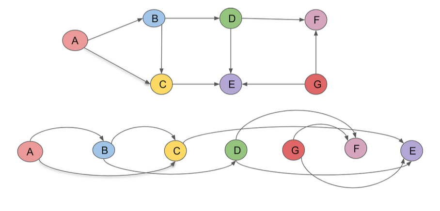
When implementing backpropagation as described above in the computational graph, the graph must be traversed in a specific order. Since the gradient of each Value depends on the gradient of its child Values, the gradient of the child Values must be completely calculated before moving to the parent. This is only possible in directed acyclic graphs, which neural networks are. To traverse the graph with the restriction imposed above, a topological sort of the directed acyclic computational graph must be found. In my implementation, this is done via a recursive method. I traverse over the nodes and compute the gradient in the order returned by sort. How a topological sort works is shown in the diagram below.

Layered Approach
The layered approach is the second approach I undertook. I did this with the expectation that this design would allow me to write the library with matrix operations to allow for parallelization and the utilization of efficient computational libraries such as numpy and cudapy. Numpy scientific computing library that runs the matrix operations efficiently on the CPU. CudaPy is an implementation of numpy that runs on the GPU.
My layered approach consists of a separate class for each type of layer. This varies from the computational graph approach in that each layer consists of a forward pass function to compute the output of the layer and a backward pass to compute the gradients. The computational graph had all functionality (i.e. forward pass and backward pass) at the individual value level rather than at the layer level. Doing this pass at the layer level allows us to compute all outputs, weight gradients and input gradients for each layer via matrix operations. This approach additionally allows for efficiency gains across another dimension, the batch size. The computational graph required passing in each input independently through the network. However, the layered approach allows for the all calculations to be done in parallel across all inputs that make up a batch.
The basic architecture of each layer is a forward pass method that takes in a batch of inputs and produces a batch of outputs, with each entry in the output batch corresponding to its entry in the inputs. The backward pass does two important calculations. The first is computing the gradients with respect to all the parameters (weights and biases) in the layer. The second is computing the gradients with respect to all the inputs. The input gradients are then returned by the backward pass and passed to the previous layer, so the previous layer has the gradients with respect to its outputs (outputs of previous layer are inputs of current layer). With this architecture, the backward pass is simply iterating over each layer, calling the backward method, getting the output and passing it to the next layer. The full implementation can be found [here.
The type of layers I implemented in this approach are fully connected, convolution layer, mean squared error and flatten. The implementation details for most of these layers are standard except for convolution and max pooling. These two layers have windowing, which is traditionally a serially implemented with for loops. However, the main benefit of this approach is parallelization via matrix operations, so I aimed to find a matrix approach. Luckily, both numpy and cudapy have an as strided function that allows for parallelized windowing by accessing the underlying bytes.
The code implementing the different layers can be found below.
from typing import Any
import numpy as np
import random
from lib.computational_graph_approach.utils import Timer

class Network:

    def set_parameters(self, params):
        for layer in self.layers:
            if layer.trainable:
                layer.params = params[:layer.params_shape[0] * layer.params_shape[1]].reshape(layer.params_shape)
                params = params[layer.params_shape[0] * layer.params_shape[1]:]

    def set_gradients(self, grads):
        for layer in self.layers:
            if layer.trainable:
                layer.grads = grads[:layer.params_shape[0] * layer.params_shape[1]].reshape(layer.params_shape)
                grads = grads[layer.params_shape[0] * layer.params_shape[1]:]

    def parameters(self):
        params = np.array([])
        grads = np.array([])
        for layer in self.layers:
            if layer.trainable:
                params = np.concatenate((params, layer.parameters()))
                grads = np.concatenate((grads, layer.gradients()))
        return params, grads

    def forward(self, inputs):
        for layer in self.layers:
            inputs = layer(inputs)
        return inputs

    def backward(self, loss_fn):
        # timer = Timer()
        prev_grad = loss_fn.backward(1.0)
        for layer in reversed(self.layers):
            # timer.start()
            prev_grad = layer.backward(prev_grad)
            # timer.stop(str(layer))
        return prev_grad

    def l2_regularization(self):
        alpha = 1e-4
        params, grads = self.parameters()
        grads += alpha * 2 * params
        self.set_gradients(grads)
        return np.sum(alpha * params * params)

    def save(self, path):
        params, _ = self.parameters()
        np.save(path, params)

    def load(self, path):
        params = np.load(path)
        self.set_parameters(params)

class FC():

    def __init__(self, num_inputs, num_outputs):
        self.num_inputs = num_inputs
        self.num_outputs = num_outputs
        self.params_shape = (num_inputs + 1, num_outputs)
        self.grads = None
        self.params = np.array([random.uniform(-1, 1) for _ in range(self.params_shape[0] * self.params_shape[1])]).reshape(self.params_shape)
        self.inputs = None
        self.trainable = True

    def __call__(self, inputs):
        self.inputs = np.column_stack((inputs, np.ones(len(inputs))))
        return np.matmul(self.inputs, self.params)

    def backward(self, prev_grad):
        # Calculate gradients for weights

        # 3D matrix of shape (batch_size, num_outputs, num_inputs + 1)
        input_matrix = np.expand_dims(self.inputs, axis=1)
        input_matrix = np.repeat(input_matrix, self.params_shape[1], axis=1)

        # 3D matrix of shape (batch_size, num_outputs, num_inputs + 1)
        prev_grad_matrix = np.expand_dims(prev_grad, axis=2)
        prev_grad_matrix = np.repeat(prev_grad_matrix, self.params_shape[0], axis=2)

        # 3D matrix of shape (batch_size, num_outputs, num_inputs + 1)
        grad_per_input = np.multiply(input_matrix, prev_grad_matrix)
        self.grads = np.transpose(np.sum(grad_per_input, axis=0))

        # Calculate gradients for inputs
        params_without_bias = self.params[:-1]
        input_grads = []
        for i in range(len(self.inputs)):
            prev_grad[i]
            input_grads.append(np.transpose(np.matmul(params_without_bias, np.transpose(prev_grad[i]))))
        return np.array(input_grads)

    def parameters(self):
        return self.params.flatten()

    def gradients(self):
        return self.grads.flatten()

class Conv2D():
    def __init__(self, input_channels, kernel_size, number_filters,
                stride=1, padding=0, compute_grads_inputs=True):
        self.input_channels = input_channels
        self.kernel_size = kernel_size
        self.number_filters = number_filters
        self.params = np.array([random.uniform(-1, 1) for _ in range(number_filters * (kernel_size * kernel_size * input_channels + 1))]).reshape(number_filters, -1)
        self.params_shape = self.params.shape
        self.grads = np.empty(self.params.shape)
        self.stride = stride
        self.padding = padding
        self.filter_shape = (number_filters, kernel_size, kernel_size, input_channels)
        self.compute_grads_inputs = compute_grads_inputs
        self.trainable = True

        # Variables during forward pass to be used for the backward pass
        self.padded_input = None
        self.sub_matrices = None

    def __call__(self, inputs):
        self.padded_input = np.pad(inputs, ((0,0),(self.padding,self.padding),(self.padding,self.padding),(0,0)), 'constant', constant_values=0)
        self.sub_matrices = self._get_conv_sub_matrices(self.padded_input)

        batch_size, output_height, output_width, num_filters = self._get_output_shape(self.padded_input)
        output = None
        for p in self.params:
            weights = p[:-1]
            bias = p[-1]
            weights = weights.reshape(self.kernel_size, self.kernel_size, self.input_channels)
            convolved = np.tensordot(self.sub_matrices, weights, axes=([2, 3, 4], [0, 1, 2]))
            convolved += bias
            convolved = convolved.reshape(batch_size, output_height, output_width, 1)
            output = convolved if output is None else np.concatenate([output, convolved], axis=-1)
        return output

    def backward(self, prev_grad):
        # Calculate gradients for weights by iterating over the filters
        ###############################################################
        for i, p in enumerate(self.params):
            # Get gradients for outputs associated with the current filter
            prev_grad_filter = prev_grad[:, :, :, i]
            prev_grad_filter = prev_grad_filter.reshape(prev_grad_filter.shape[0], prev_grad_filter.shape[1] * prev_grad_filter.shape[2])
            # Get gradients for weights by multiplying the inputs by the gradients of the outputs
            weights_grads = np.einsum('ijklm,ij->ijklm', self.sub_matrices, prev_grad_filter)
            # Sum the gradients across the batch
            weights_grads = np.reshape(weights_grads, (weights_grads.shape[0]*weights_grads.shape[1], -1))
            weights_grads = np.sum(weights_grads, axis=0)
            # Get the gradient for the bias by summing the gradients of the outputs across the batch
            bias_grad = np.sum(prev_grad_filter.flatten())
            # Update the weights and bias
            self.grads[i] = np.append(weights_grads, bias_grad)

        # Calculate gradients for inputs
        ###############################################################
        if self.compute_grads_inputs:
            batch_size, output_height, output_width, num_filters = self._get_output_shape(self.padded_input)
            filters = self.params[:, :-1].reshape(self.filter_shape)
            filter_masks = []

            input_num_rows = self.padded_input.shape[1]
            input_num_cols = self.padded_input.shape[2]

            for i in range(output_height):
                for j in range(output_width):
                    curr_filter_mask = np.pad(filters, ((0,0),(i * self.stride, input_num_rows - (i*self.stride + self.kernel_size)),(j * self.stride, input_num_cols - (j*self.stride + self.kernel_size)),(0,0)), 'constant', constant_values=0)
                    filter_masks.append(curr_filter_mask)

            # (output_width * output_height, num_filters, input_rows, input_cols, input_channels)
            filter_masks = np.array(filter_masks)
            # (1, output_width * output_height, num_filters, input_rows, input_cols, input_channels)
            filter_masks = np.expand_dims(filter_masks, axis=0)
            # (batch_size, output_width * output_height, num_filters, input_rows, input_cols, input_channels)
            filter_masks = np.repeat(filter_masks, batch_size, axis=0)
            # (batch_size, output_width * output_height, num_filters)
            prev_grad_shaped = prev_grad.reshape(prev_grad.shape[0], prev_grad.shape[1]*prev_grad.shape[2], prev_grad.shape[3])
            # (batch_size, output_width * output_height, num_filters, input_rows, input_cols, input_channels)
            # ** Need to trim if there is padding **
            backward_grads = np.einsum('ijk,ijklmn->ijklmn', prev_grad_shaped, filter_masks)
            # Sum for gradients
            return np.sum(backward_grads, axis=(1,2))
        else:
            return None

    def _get_output_shape(self, inputs):
        batch_size = inputs.shape[0]
        input_height = inputs.shape[1]
        input_width = inputs.shape[2]
        output_width = int((input_width + 2*self.padding - self.kernel_size) / self.stride + 1)
        output_height = int((input_height + 2*self.padding - self.kernel_size) / self.stride + 1)
        return batch_size, output_height, output_width, self.number_filters

    def _get_conv_sub_matrices(self, inputs):
        # Get the sub matrices for the convolution
        item_size = inputs.itemsize
        batch_size = inputs.shape[0]
        input_height = inputs.shape[1]
        input_width = inputs.shape[2]
        input_channels = inputs.shape[3]

        # Get the shape of the sub matrices
        kernel_size = self.kernel_size
        __, output_height, output_width, _ = self._get_output_shape(inputs)
        shape = (batch_size, output_height, output_width, kernel_size, kernel_size, input_channels)

        # Get strides of the sub matrices
        channel = item_size
        column = channel * input_channels
        row = column * input_width
        horizontal_stride = self.stride * column
        vertical_stride = self.stride * row
        batch = input_height * input_width * column
        stride_shape = (batch, vertical_stride, horizontal_stride, row, column, channel)

        # Get the sub matrices
        sub_matrices = np.lib.stride_tricks.as_strided(inputs, shape=shape, strides=stride_shape)

        # Combine output height and output width
        sub_matrices = np.reshape(sub_matrices, (batch_size, output_height * output_width, kernel_size, kernel_size, input_channels))

        return sub_matrices

    def parameters(self):
        return self.params.flatten()

    def gradients(self):
        return self.grads.flatten()


class MaxPool2D():

    def __init__(self, kernel_size):
        self.kernel_size = kernel_size
        self.stride = kernel_size
        self.trainable = False
        self.grads = None

        # Variables during forward pass to be used for the backward pass
        self.input = None
        self.sub_matrices = None

    def __call__(self, input):
        self.input = input
        sub_matrices = self._get_pool_sub_matrices(self.input)
        self.sub_matrices = sub_matrices
        batch_size, output_height, output_width, output_channels = self._get_output_shape(self.input)
        # Reshape from (batch_size, num_sub_matrices, kernel_size, kernel_size, input_channels) to (batch_size * num_sub_matrices, kernel_size, kernel_size, input_channels)
        sub_matrices = np.reshape(sub_matrices, (sub_matrices.shape[0] * sub_matrices.shape[1], sub_matrices.shape[2], sub_matrices.shape[3], sub_matrices.shape[4]))
        # Get the max value for each sub matrix
        max_pool = np.max(sub_matrices, axis=(1,2))
        # Reshape from (batch_size * num_sub_matrices, input_channels) to (batch_size, output_height, output_width, output_channels)
        # Output channels is the same as input channels for max pooling
        output = np.reshape(max_pool, (batch_size, output_height, output_width, output_channels))
        return output


    def backward(self, prev_grad):
        pass


    def _get_output_shape(self, inputs):
        batch_size = inputs.shape[0]
        input_height = inputs.shape[1]
        input_width = inputs.shape[2]
        input_depth = inputs.shape[3]

        output_width = int((input_width - self.kernel_size) / self.stride + 1)
        output_height = int((input_height - self.kernel_size) / self.stride + 1)
        return batch_size, output_height, output_width, input_depth

    def _get_pool_sub_matrices(self, inputs):
        # Get the sub matrices for the pooling
        item_size = inputs.itemsize
        batch_size = inputs.shape[0]
        input_height = inputs.shape[1]
        input_width = inputs.shape[2]
        input_channels = inputs.shape[3]

        # Get the shape of the sub matrices
        kernel_size = self.kernel_size
        __, output_height, output_width, _ = self._get_output_shape(inputs)
        shape = (batch_size, output_height, output_width, kernel_size, kernel_size, input_channels)

        # Get strides of the sub matrices
        channel = item_size
        column = channel * input_channels
        row = column * input_width
        horizontal_stride = self.stride * column
        vertical_stride = self.stride * row
        batch = input_height * input_width * column
        stride_shape = (batch, vertical_stride, horizontal_stride, row, column, channel)

        # Get the sub matrices
        sub_matrices = np.lib.stride_tricks.as_strided(inputs, shape=shape, strides=stride_shape)

        # Combine output height and output width
        sub_matrices = np.reshape(sub_matrices, (batch_size, output_height * output_width, kernel_size, kernel_size, input_channels))

        return sub_matrices

class Flatten():
    def __init__(self):
        self.inputs_shape = None
        self.trainable = False

    def __call__(self, inputs):
        self.inputs_shape = inputs.shape
        return np.reshape(inputs, (inputs.shape[0], -1))

    def backward(self, prev_grad):
        return np.reshape(prev_grad, self.inputs_shape)

class ReLU():

    def __init__(self):
        self.inputs = None
        self.trainable = False

    def __call__(self, inputs):
        self.inputs = inputs
        return np.maximum(self.inputs, 0)

    def backward(self, prev_grad):
        input_grads = prev_grad * (self.inputs > 0)
        return input_grads

class MSE():

    def __init__(self):
        self.inputs = None
        self.targets = None
        self.trainable = False

    def __call__(self, inputs, targets):
        self.inputs = inputs
        self.targets = targets
        return np.mean(np.square(inputs - targets).flatten())

    def backward(self, prev_grad):
        grads = 2 * prev_grad * (self.inputs - self.targets) / len(self.inputs.flatten())
        return grads

class SVM():

    def __init__(self):
        self.inputs = None
        self.targets = None
        self.trainable = False

    def __call__(self, inputs, targets):
        self.inputs = inputs
        self.targets = targets
        return np.mean(np.maximum(0, 1 - inputs * targets))

    def backward(self, prev_grad):
        input_grads = prev_grad * -self.targets * (self.inputs * self.targets < 1) / len(self.inputs)
        return input_grads
Comparison
I used both implementations to train a DQN to solve the Cart Pole problem. The results table below show that layered approach running on the CPU is fastest by 100x. It is faster than the computational graph approach as expected, however it is unexpectedly slower than the layered approach on the GPU. I suspect it may be due to the time it takes to move the data from the CPU to the GPU the number of times required for training the RL agent.
| Method | Forward Pass (ms) | Backward Pass (ms) | Total Time - 1000 iterations (s) |
|---|---|---|---|
| Computational Graph | 2.47 | 0.66 | 99.95 |
| Layered (numpy/CPU) | 0.011 | 0.048 | 1.57 |
| Layered (cupy/GPU) | 0.31 | 0.57 | 28.35 |
RL Agent
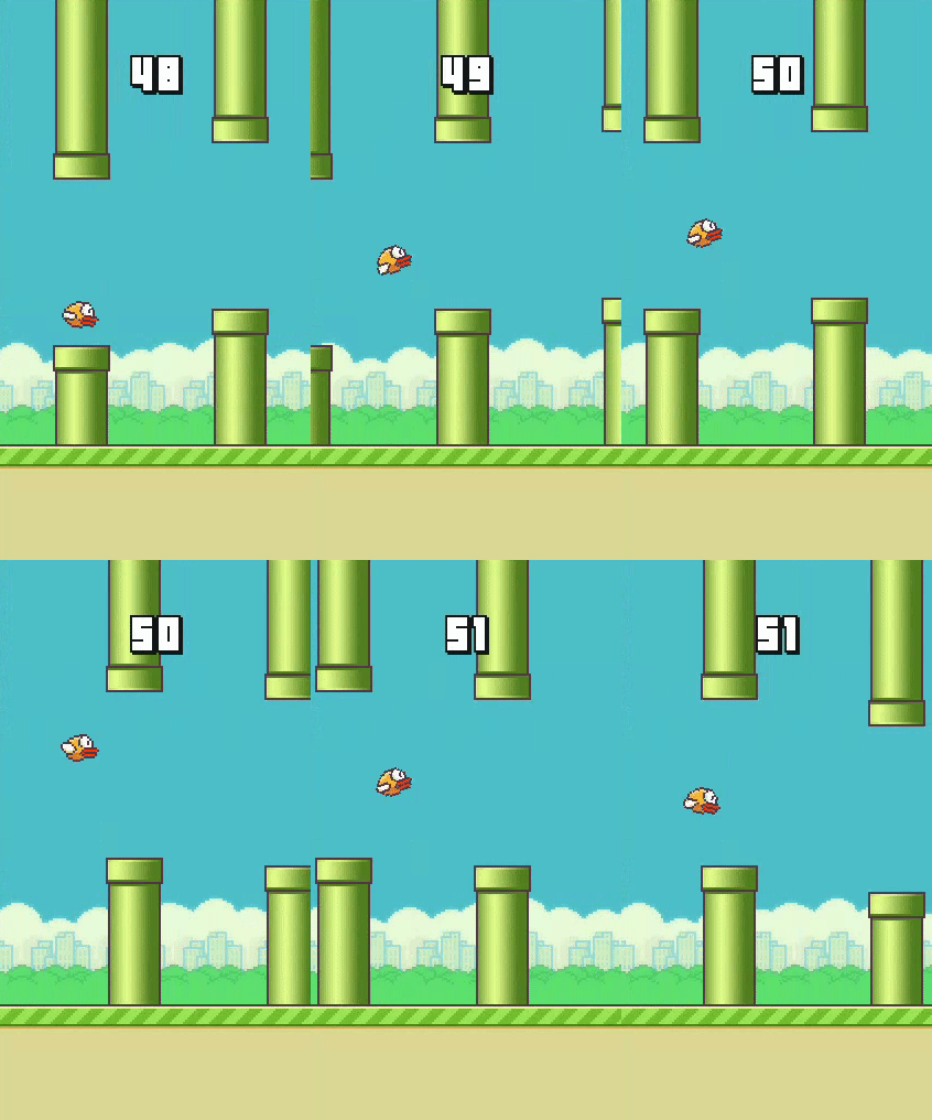
I built an RL agent to play Flappy Bird. Flappy Bird is a game that requires the player to have a bird looking sprite navigate through gaps in pipes. The sprite has a constant x velocity as it moves towards the pipes. The player has the ability to apply a force in the y direction. The goal is for the player to time the application of the force to navigate through the gaps between the pipes for as long as possible. The code for running the agent can be found here.
Environment
For Flappy Bird, I used an environment following the gym API to train and evaluate my agent.
Observation Space
- x difference between the bird and the gap in the next pipe
- y difference between the bird and the gap in the next pipe
Action Space
- 0 applying no force and 1 applying a set force.
Reward
- A value of 1 returned every time step the bird did not crash.
Termination Condition
- Crashing into a pipe or ground or going above the top of the screen
One thing worth pointing out is that the Markov assumption does not fully hold for the state because the velocity of the bird is not included. I only have positional information. However, this proves to be sufficient, but may reduce the efficiency of the training.
DQN Agent
DQN Algorithm
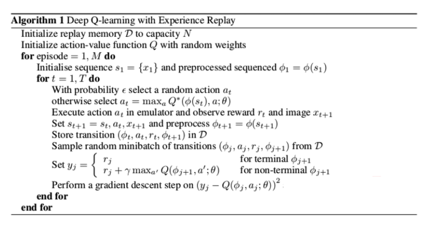
The DQN agent uses a Deep Q Network (DQN) to learn a policy. To understand a deep Q network, I will explains its foundation, which is Q-learning. Q-learning works with the assumption that states/observations follow the Markov property. This means that the state encapsulates all information about the environment that allows for the agent to find an optimal action. It is centered around the Q function. The Q function takes in the state and action and produces a value. The higher the values, the better the state action pair. In Q-learning, the goal is to learn this Q function. From this Q function, an agent can find the optimal action when given a state by finding the action that returns the highest Q value when paired with the state. The Q function is ultimately learned via repeated Bellman updates to the Q function. As the equation below shows, the Q value for the current state-action pair, is the max Q value for the next state multiplied by discount factor (γ), added to the reward that was returned for getting to the next state. Repeatedly running this update with collected returns an optimal Q function. For a DQN, this Q function is represented by a neural network and is updated via a gradient step. This gradient step is taken at the end of each episode on a batch of experiences saved from previous episodes. This buffer of saved experiences is called replay memory. The full algorithm for a DQN is shown below.
$ Q_{i+1}(s, a) = \mathbb{E}_{s' \sim e} [r + \gamma \max_{a'} Q_i(s^{\prime}, a^{\prime}) | s, a] $
Bellman Optimality Equation

DQN Algorithm
Neural Network and Training Parameters
Neural Network Architecture: Used the following neural network architecture below with a mean squared loss function, the epsilon decay rate function below and a sampling of random actions to weighted 75 percent towards applying no force and 25 percent towards applying a force. This allowed for more efficient exploration of the space because apply a force as often as not applying one quickly results in crashes in the beginning.
- Fully Connected (in: 2, out: 64)
- ReLU
- Fully Connected (in: 64, out: 128)
- ReLU
- Fully Connected (in: 128, out: 2)
$ \text{epsilon\_decay} = {\sqrt[num\_episodes]{\frac{0.01}{\epsilon}}} $
Epsilon Decay Rate Function
Training Parameters
- Discount factor (γ): 0.95
- Batch size: 32
- Leanning rate: 0.001
- Replay memory size: 2000
Results
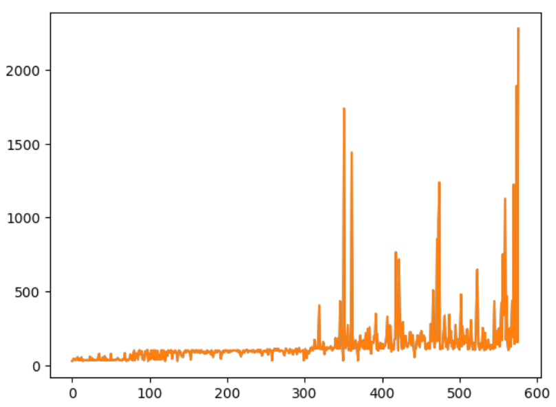
After training for 576,000 episodes (2 hours on a personal PC), the network converged at a solution for an agent that averaged over 2000 time steps when playing Flappy Bird. This results in an average score of navigating through 30 pipes. While this is not super human performance, it shows that the agent can play the game. With more training time, the agent would be able to play at super human levels. The graph below plots the average episode length of running the agent for 10 episodes after every 1000 episodes of training. The code for training the agent can be found here.
