May 2023 - August 2024
Stanford Vision Lab
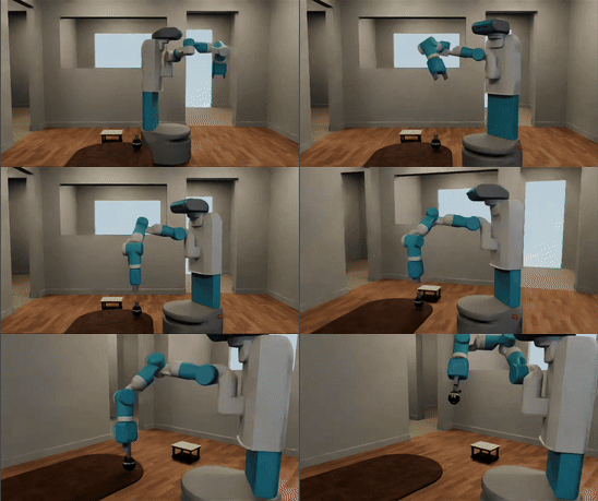
I was a student researcher at SVL developing motion primitives for a robot in a simulation environment. These motion primitives are Python functionality that execute robotic actions to accomplish basic tasks. These tasks consist of grasping and placing an object, open and closing doors/drawers and navigating. The purpose of developing these primitives is to aid researchers in accomplishing the BEHAVIOR-1K benchmark using the OmniGibson simulation environment built on NVIDIA Omniverse and Isaac Sim. My work is included in BEHAVIOR-1K paper here.
I, along with a few others, took two approaches to building out these primitives. Our first approach was using the full observability of the environment to develop algorithmic primitives. After completing our first approach, we were dissatisfied with its ability generalize to the significantly varied tasks in the BEHAVIOR-1K benchmark. So, we then used some of the fundamental functionality developed in our first approach to aid our second approach. This approach is using reinforcement learning to learn a selection of robotic actions.
References:
Cem Gokmen, Ph.D @ SVL, cgokmen@stanford.edu (Primary)
Rouhan Zhang, Postdoctoral Researcher @ SVL, zharu@stanford.edu (Secondary)
Algorithmic Primitives
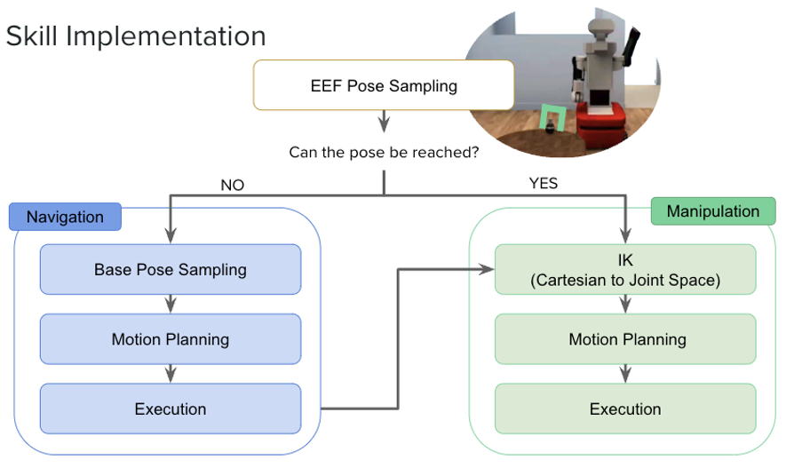
The algorithmic implementation for the motion primitives follow a common logical flow. The steps are the following and are illustrated in the diagram below:
- Sample among valid end effector (EEF) poses generated
- Test whether the sampled pose is within the robot’s reach by checking whether IsaacSim’s IK solver returns a valid arm configuration for that pose
- If it returns an invalid configuration, we then execute our navigation flow. Otherwise, execute the manipulation flow.
- Navigation or Manipulation flow
Navigation Flow
The navigation flow consists of first sampling base poses in SE(2) near the proposed EEF pose. Every pose is checked to be collision free and within the robot’s reach. Once a valid base position is found, we pass it to the motion planner. We use OMPL for motion planning with a custom motion validator. The motion planner uses RRT to explore the search space and find a path. The custom motion validator checks for validity between two points in RRT by validating a motion where the robot turns to face the goal from the initial orientation, moves in a line to the goal, and turns to face the goal’s final orientation is collision free. This custom motion validator needed to be implemented because the default motion checking in RRT is having the robot translate and rotate simultaneously to a goal, which is not how the robot moves in our primitives implementation. Finally, once a valid path is found, the robot executes this path. The code for find the valid path described is below.
def plan_base_motion(
    robot,
    end_conf,
    context,
    planning_time=15.0,
):
    """
    Plans a base motion to a 2d pose

    Args:
        robot (omnigibson.object_states.Robot): Robot object to plan for
        end_conf (Iterable): [x, y, yaw] 2d pose to plan to
        context (PlanningContext): Context to plan in that includes the robot copy
        planning_time (float): Time to plan for

    Returns:
        Array of arrays: Array of 2d poses that the robot should navigate to
    """
    from ompl import base as ob
    from ompl import geometric as ompl_geo

    class CustomMotionValidator(ob.MotionValidator):

        def __init__(self, si, space):
            super(CustomMotionValidator, self).__init__(si)
            self.si = si
            self.space = space

        def checkMotion(self, s1, s2):
            if not self.si.isValid(s2):
                return False

            start = th.tensor([s1.getX(), s1.getY(), s1.getYaw()])
            goal = th.tensor([s2.getX(), s2.getY(), s2.getYaw()])
            segment_theta = self.get_angle_between_poses(start, goal)

            # Start rotation
            if not self.is_valid_rotation(self.si, start, segment_theta):
                return False

            # Navigation
            dist = th.norm(goal[:2] - start[:2])
            num_points = math.ceil(dist / m.DIST_DIFF) + 1
            nav_x = th.linspace(start[0], goal[0], num_points).tolist()
            nav_y = th.linspace(start[1], goal[1], num_points).tolist()
            for i in range(num_points):
                state = create_state(self.si, nav_x[i], nav_y[i], segment_theta)
                if not self.si.isValid(state()):
                    return False

            # Goal rotation
            if not self.is_valid_rotation(self.si, [goal[0], goal[1], segment_theta], goal[2]):
                return False

            return True

        @staticmethod
        def is_valid_rotation(si, start_conf, final_orientation):
            diff = _wrap_angle(final_orientation - start_conf[2])
            direction = th.sign(diff)
            diff = abs(diff)
            num_points = math.ceil(diff / m.ANGLE_DIFF) + 1
            nav_angle = th.linspace(0.0, diff, num_points) * direction
            angles = nav_angle + start_conf[2]
            for i in range(num_points):
                state = create_state(si.getStateSpace(), start_conf[0], start_conf[1], angles[i])
                if not si.isValid(state()):
                    return False
            return True

        @staticmethod
        # Get angle between 2d robot poses
        def get_angle_between_poses(p1, p2):
            segment = []
            segment.append(p2[0] - p1[0])
            segment.append(p2[1] - p1[1])
            return th.arctan2(segment[1], segment[0])

    def create_state(space, x, y, yaw):
        x = float(x)
        y = float(y)
        yaw = float(yaw)
        state = ob.State(space)
        state().setX(x)
        state().setY(y)
        state().setYaw(_wrap_angle(yaw))
        return state

    def state_valid_fn(q):
        x = q.getX()
        y = q.getY()
        yaw = q.getYaw()
        pose = ([x, y, 0.0], T.euler2quat((0, 0, yaw)))
        return not set_base_and_detect_collision(context, pose)

    def remove_unnecessary_rotations(path):
        """
        Removes unnecessary rotations from a path when possible for the base where the yaw for each pose in the path is in the direction of the
        the position of the next pose in the path

        Args:
            path (Array of arrays): Array of 2d poses

        Returns:
            Array of numpy arrays: Array of 2d poses with unnecessary rotations removed
        """
        # Start at the same starting pose
        new_path = [path[0]]

        # Process every intermediate waypoint
        for i in range(1, len(path) - 1):
            # compute the yaw you'd be at when arriving into path[i] and departing from it
            arriving_yaw = CustomMotionValidator.get_angle_between_poses(path[i - 1], path[i])
            departing_yaw = CustomMotionValidator.get_angle_between_poses(path[i], path[i + 1])

            # check if you are able to make that rotation directly.
            arriving_state = (path[i][0], path[i][1], arriving_yaw)
            if CustomMotionValidator.is_valid_rotation(si, arriving_state, departing_yaw):
                # Then use the arriving yaw directly
                new_path.append(arriving_state)
            else:
                # Otherwise, keep the waypoint
                new_path.append(path[i])

        # Don't forget to add back the same ending pose
        new_path.append(path[-1])

        return new_path

    pos = robot.get_position()
    yaw = T.quat2euler(robot.get_orientation())[2]
    start_conf = (pos[0], pos[1], yaw)

    # create an SE(2) state space
    space = ob.SE2StateSpace()

    # set lower and upper bounds
    bbox_vals = []
    for floor in filter(lambda o: o.category == "floors", robot.scene.objects):
        bbox_vals += floor.aabb[0][:2].tolist()
        bbox_vals += floor.aabb[1][:2].tolist()
    bounds = ob.RealVectorBounds(2)
    bounds.setLow(min(bbox_vals))
    bounds.setHigh(max(bbox_vals))
    space.setBounds(bounds)

    # create a simple setup object
    ss = ompl_geo.SimpleSetup(space)
    ss.setStateValidityChecker(ob.StateValidityCheckerFn(state_valid_fn))

    si = ss.getSpaceInformation()
    si.setMotionValidator(CustomMotionValidator(si, space))
    # TODO: Try changing to RRTConnect in the future. Currently using RRT because movement is not direction invariant. Can change to RRTConnect
    # possibly if hasSymmetricInterpolate is set to False for the state space. Doc here https://ompl.kavrakilab.org/classompl_1_1base_1_1StateSpace.html
    planner = ompl_geo.RRT(si)
    ss.setPlanner(planner)

    start = create_state(space, start_conf[0], start_conf[1], start_conf[2])
    print(start)

    goal = create_state(space, end_conf[0], end_conf[1], end_conf[2])
    print(goal)

    ss.setStartAndGoalStates(start, goal)
    if not state_valid_fn(start()) or not state_valid_fn(goal()):
        return

    solved = ss.solve(planning_time)

    if solved:
        # try to shorten the path
        ss.simplifySolution()
        sol_path = ss.getSolutionPath()
        return_path = []
        for i in range(sol_path.getStateCount()):
            x = sol_path.getState(i).getX()
            y = sol_path.getState(i).getY()
            yaw = sol_path.getState(i).getYaw()
            return_path.append([x, y, yaw])
        return remove_unnecessary_rotations(return_path)
    return None
Manipulation Flow
The manipulation phase of the primitives consists similarly of three steps.
- Use IK to find a valid arm configuration to reach the EEF pose
- Use the arm configuration into a default OMPL motion planner bounded by the joint limits of the robot to find a path in configuration space.
- Execute the computed path using our joint controller.
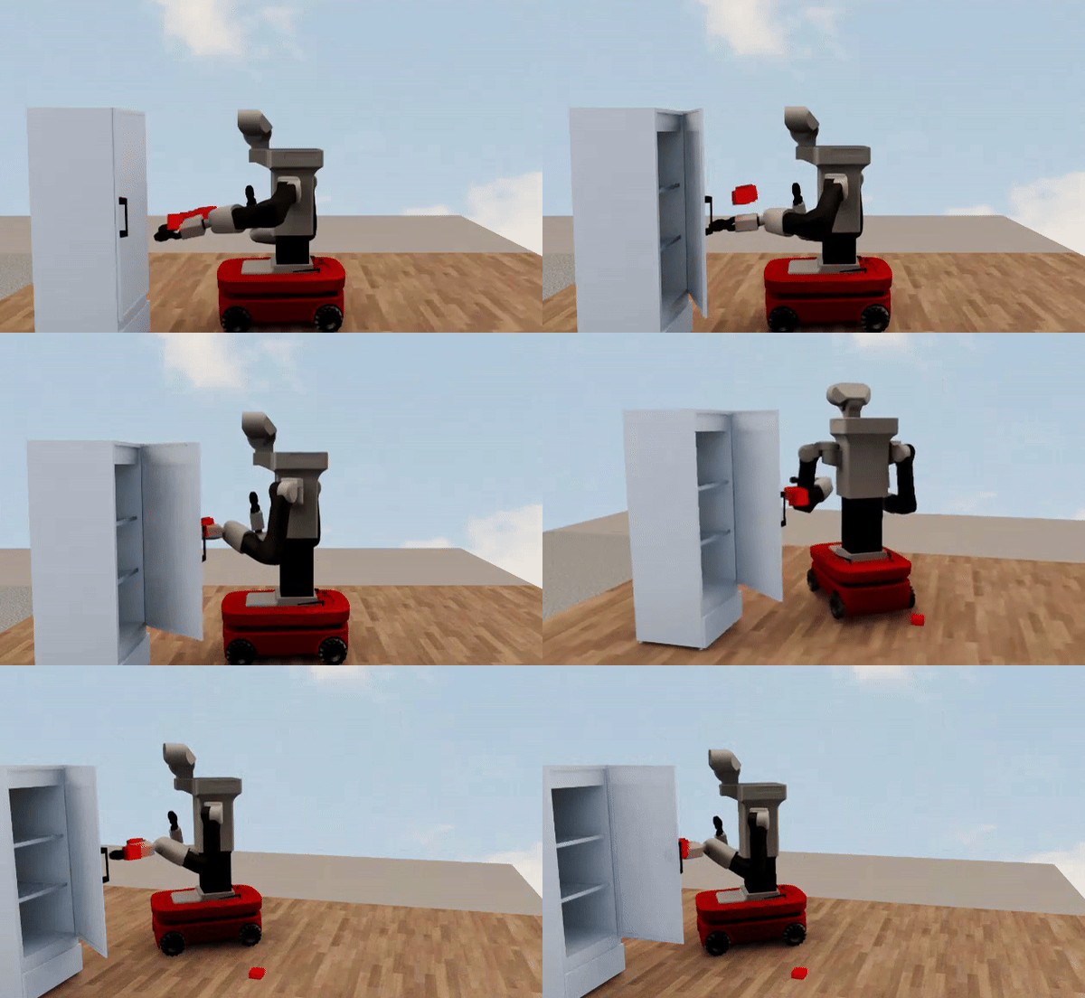
After this manipulation phase, every primitive has its own custom execution of grasping, closing, opening, etc. Below is an example of opening a door.
Collision Detection
The main technical feature in our algorithmic primitives implementation is the collision detection, specifically during planning where the robot is moved around the environment to check for collisions. Using the simplest simulation option of saving the current simulator state, setting the robot at a specific arm configuration or 2d pose, taking a simulator step, then have the simulator check for collisions and finally resetting the original saved state proved to be prohibitively slow. We chose to implement a method that used a copy of the collision meshes of the robot and check for overlaps with the collision meshes of other objects in the environment to detect a collision WITHOUT taking a simulation step. This increased planning speed by 20x. Our collision detection method is implemented separately for navigation and manipulation.
Navigation
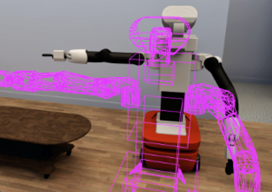
When the simulation environment spawns, we create copies of the robot’s collision meshes and store their transforms relative to the base of the robot. Then for collision detection in navigation, we reassemble the robot at a specified location by using the relative transforms for the meshes to calculate the poses for the meshes in the world frame to construct the robot as shown in the image below. Once this is completed, we then check to see if the meshes overlap with the meshes of other objects in the scene. However, an additional complication is introduced when the robot is holding an object. In this case, we ignore overlaps between the end effector of the robot and the object. Lastly, we also copy the meshes of the object in the hand and check that it does not overlap with any other invalid objects in the scene, because the object in the hand should function as part of the robot.
Manipulation
For manipulation, collision detection gets additionally complicated. This is because manipulation requires setting different arm configurations for the arm, then checking for overlap. To address this, we use a forward kinematics solver in Omniverse that when given the joint configurations, will return the relative poses of the meshes of the robot to create that configuration. We then compute the world pose for the meshes using the relative poses and the pose of the robot, set the meshes to those poses and finally check for overlap in a similar manner described above. The only difference is that we add the robot meshes to the list of invalid meshes. This is because invalid arm configurations include those where the robot collides with itself.
Reinforcement Learning
Our second approach is using reinforcement learning to develop the primitives. Since RL is sample inefficient, it requires high frames per second (FPS) from our simulation to collect enough data in a reasonable time. To get this high FPS, we engineered two solutions. The first is using gRPC to allow for running multiple environments in parallel on a distributed cluster and the second is running multiple scenes in a single environment on a single node.
gRPC Parallel Environments
In RL, parallelizable environments are wrapped in a vector environment that allows an RL library step them simultaneously to speed up training. We created a custom environment wrapper that communicates via gRPC between the multiple environments we manually spin up (code). The overall architecture is that we have a learner script (code) that spins up a registration server and waits for workers to connect. We then run a worker script that spins up multiple RL environments that have an associated IP, accept an action to run and return an observation (code). The worker script sends the IPs to the registration server. Now the learner script can create our vectorized environment that can accept an array of actions, send them via a client-server connection to the environment workers and return an array of observations from the environment workers.
OmniGibson Parallel Environments
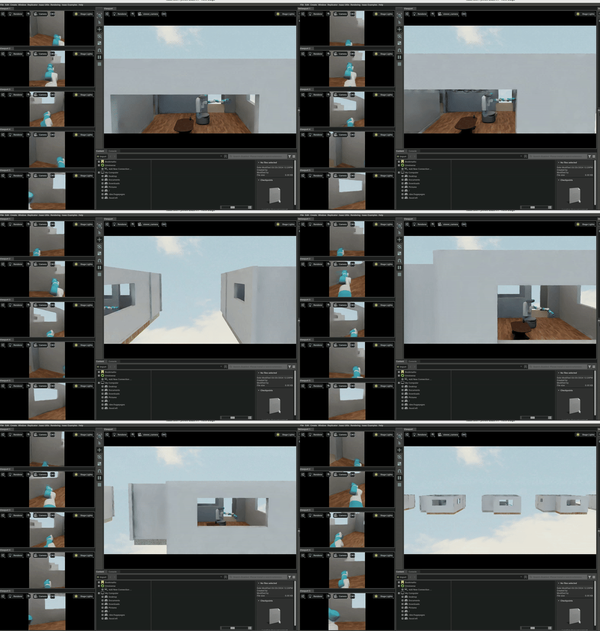
The gRPC set up can have some network delays and is cumbersome to work with, so we later implemented a native version of multiple environments in OmniGibson. Since OmniGibson is built on IsaacSim, it allows for the creation of multiple scenes in a single environment. We refactored OmniGibson to be vectorized to support this. The graphic below shows the result and the PR can be found here. The result is an 5-10x increase in FPS to around 250 FPS.
RL Environment
In addition to our engineering efforts, we setup a simple RL environment to learn grasping. Key aspects of this environment are the following:
Observation Space
- Joint positions of the robot arm
- Relative position of the center of the robot base the the centroid of the object to grasp
- Relative position of the center of the bounding box for the end effector (EEF) and the centroid fo the object to grasp
Action Space
- Delta joint positions for the robot arm that are fed to our joint controller
Reward
The reward function for grasping is the sum of a distance reward, regularization reward and a collision penalty.
The distance reward is defined by 4 cases that are determined by the state before an action and the following state (i.e. current state). The table below outlines these states:
| Previous State | Current State (After action) | Reward |
|---|---|---|
| Not grasping object | Not grasping object | $e^{(\text{distance between EEF and object} \times -1)} \times \text{dist\_coeff}$ |
| Not grasping object | Grasping object (picked object) | $e^{(\text{distance between robot center and object} \times -1)} \times \text{dist\_coeff} + \text{grasp\_reward}$ |
| Grasping object | Not grasping object (dropped object) | $e^{(\text{distance between EEF and object} \times -1)} \times \text{dist\_coeff}$ |
| Grasping object | Grasping object | $e^{(\text{distance between robot center and object} \times -1)} \times \text{dist\_coeff} + \text{grasp\_reward}$ |
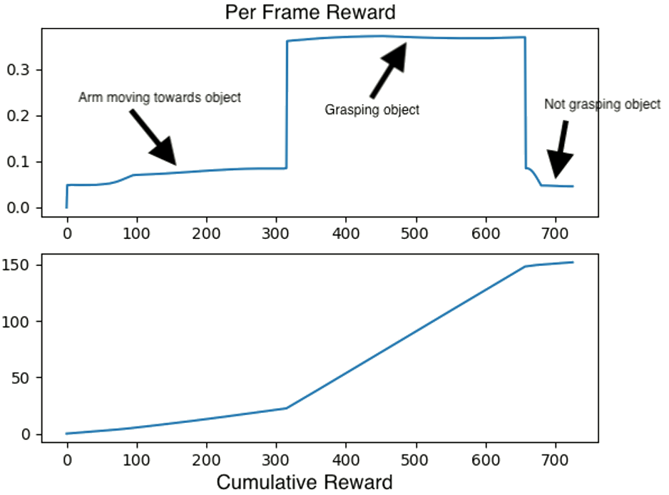
The reward function is shaped in a way where the closer the end effector is to the object when it is not holding an object, the higher the reward. Once the robot grasps the object, the lower the moment of inertia for the robot object pair, the higher the reward. A graph of the reward per frame and cumulative distance reward for a robot grasping, then dropping the desired object is shown below.
The regularization reward is a penalty that subtracts an amount proportional to the applied joint efforts and the amount the EEF moves during a step. This will discourage unnecessary movements.
The collision penality is an amount subtracted everytime the robot collides with something in the environment to discourage collisions.
Termination Condition
The termination condition is when the object is in the grasp of the end effector or 400 timesteps have passed.
Resetting Condition
To learn general grasping, we reset the robot to randomized arm configurations and robot base poses around the object. To randomize the arm configuration, we generate random configurations and use our collision checking functionality to find a valid starting configuration. We do the same for the base pose where we sample around the object to grasp and find a pose that places the robot within the reach of the object and is collision free.
Results
So far we have gotten mediocre results in grasping where the arm does grasp the object, but is jittery and takes a circuitous route to the object. We need to run more experiments, which is only tractable with higher frames per second. To achieve this, we plan on tensorizing as much as we can in OmniGibson so it is taking advantage of the GPU as much as possible.